Finding good information on how filters work, what the different types of filters mean, and how you should filter your data is hard. Lots of explanations only make sense if you have a year or two of electrical engineering education, and most of the rest are just a list of rules of thumb. I want to try to get you to a place where you can test your own filter settings, and show you the importance of the rules of thumb without going into the relatively complex math that is often used to explain filters. Warning: a lot of the code I’m going to use requires the Matlab Signal Processing Toolbox. If you don’t have it, you wont be able to execute the code yourself, but hopefully you’ll still be able to follow along with the logic.
What is a filter?
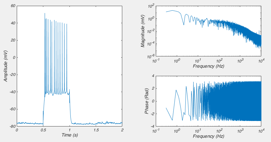
Fig 1. On the left is a recording from a neuron shown in the “time domain”. The two graphs on the right show the same recording in the “frequency domain”
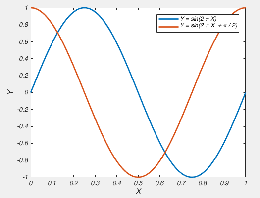
Fig 2. A graph of Y = sin(2π X) and a graph of Y = sin(2πX + π/2) have the same frequency components, but different phases
There are a huge variety of filters, but one of the simplest ways of dividing them up is to consider what signals they don’t affect, i.e. what signals they let pass through them. So a low-pass filter lets through low frequency signals and a high-pass filter lets through high frequency data. There are also band-pass filters which only let through signals in a particular frequency range and to break convention, band-stop filters, which stop signals inside a particular frequency range. The frequency at which the signal begins to be filtered is called the “corner frequency” or the “cut-off frequency”. When we describe the actions of a filter, we are often show it’s frequency response, which is shows you what the filter does to various frequency components of your data. This can be estimated by applying the filter to your data, viewing it in the frequency domain and then dividing that by your original signal in the frequency domain. However, as your data doesn’t usually contain all frequency components, it better to create white noise, which is a signal that has the same amount of power in all frequency components. We can convert data to the frequency domain by using the Fourier transform (which I’ve talked about before here). In code, that looks like this.
signal = randn(1000,1); %Create white noise
dt = 0.5; %dt is the time between samples
time = 1:dt:1000 ; %create time base

%% Filter the data
%Make a simple running average filter
%Take the mean of the original data in a window
%of the data tempC(i:i+window)
%I know there are faster ways of doing this.

tempC_filt = zeros(size(signal));

window = 5;
for i = 1:length(signal)
end_idx = i+window;
if end_idx > length(signal)
    end_idx = length(signal);
end
tempC_filt(i) = mean(signal(i:end_idx));
end

%% Now convert data to frequency domain

nfft = 2^nextpow2(length(signal)); %FFTs are faster if you perform them
                                  %on power of 2 lengths vectors

f = (1/dt)/2*linspace(0,1,nfft/2+1)'; %Create Frequency vector'

dft      = fft(signal, nfft)/(length(signal)/2); % take the FFT of original
dft_filt = fft(tempC_filt, nfft)/(length(tempC_filt)/2); %take FFT of filters
mag = abs(dft(1:nfft/2+1));                     %Calculate magnitude
mag_filt = abs(dft_filt(1:nfft/2+1));           %Calculate magnitude

loglog(f, mag_filt./mag)
xlabel('Frequency (Hz)')
ylabel('Signal Out / Signal In')
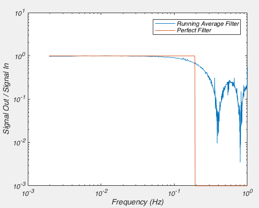
Fig 3. The frequency response of a running average filter.
Now I’ve said a perfect filter doesn’t want to alter signals in the pass-band, and by looking at the graph above, it might appear that so long as you are below about 0.1 Hz you wont affect the signal, but as I alluded to before, we need to consider what the filter does to the phase. We can achieve that by adding only a few more lines to our above code.
signal = randn(1000,1); %Create random time series data
dt = 0.5; %dt is the time between samples
time = 1:dt:1000 ; %create time base

%% Filter the data
%Make a simple running average filter
%Take the mean of the original data in a window
%of the data tempC(i:i+window)
%I know there are faster ways of doing this.

tempC_filt = zeros(size(signal));

window = 5;
for i = 1:length(signal)
end_idx = i+window;
if end_idx > length(signal)
    end_idx = length(signal);
end
tempC_filt(i) = mean(signal(i:end_idx));
end

%% Now convert data to frequency domain

nfft = 2^nextpow2(length(signal)); %FFTs are faster if you perform them
                                  %on power of 2 lengths vectors

f = (1/dt)/2*linspace(0,1,nfft/2+1)'; %Create Frequency vector'

dft      = fft(signal, nfft)/(length(signal)/2); % take the FFT of original
dft_filt = fft(tempC_filt, nfft)/(length(tempC_filt)/2); %take FFT of filters
mag = abs(dft(1:nfft/2+1));                     %Calculate magnitude
mag_filt = abs(dft_filt(1:nfft/2+1));           %Calculate magnitude

phase = angle(dft(1:nfft/2+1));
phase_filt = angle(dft_filt(1:nfft/2+1));

%% Create an ideal filter frequency response
mag_perf = ones(size(mag_filt));
mag_perf(100:end) = 10^-3;

subplot(1,2,1)
loglog(f, mag_filt./mag, f, mag_perf)
xlabel('Frequency (Hz)')
ylabel('Signal Out / Signal In')
legend('Running Average Filter', 'Perfect Filter')

subplot(1,2,2)
semilogx(f, unwrap(phase-phase_filt));
xlabel('Frequency (Hz)')
ylabel('Phase Shift (Rad)')
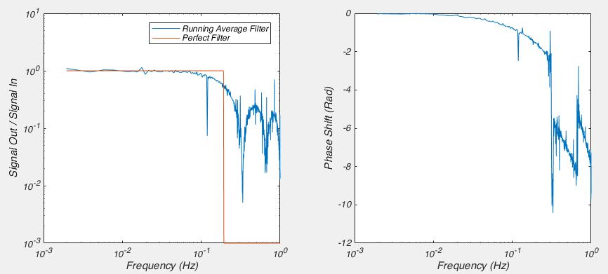
Fig 4. Magnitude and Phase response of a running average filter
Filter Poles
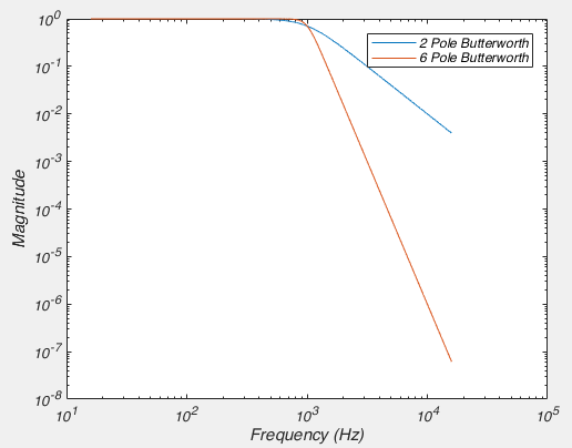
Fig 5. How the frequency response of a filter varies with the number of poles.
Another way of describing a filter is by the number of “poles” it has. I’m not going to explain to you what a pole is, because it comes from the mathematical analysis of filters, and ultimately, it is irrelevant for understanding what the consequence of the filter is. Simply put a filter with more poles attenuates frequencies more heavily for each Hz you go up. Here a figure will paint a thousand words, so see fig 5. We can create that figure with the below code.
%All our filters will have a corner
%frequence (fc) of 1000 Hz
fc = 1000; % Corner Frequency of

[b2pole,a2pole] = butter(2,2*pi*fc,'s'); %Create a 2 pole butterworth filter
[h2pole,freq2] = freqs(b2pole,a2pole,4096);     %Calculate Frequency Response

[b6pole,a6pole] = butter(6,2*pi*fc,'s'); %Create a 2 pole butterworth filter
[h6pole,freq6] = freqs(b6pole,a6pole,4096);     %Calculate Frequency Response

%Plot frequency response
loglog(freq2/(2*pi),abs(h2pole));
hold on
loglog(freq6/(2*pi),abs(h6pole));
xlabel('Frequency (Hz)');
ylabel('Magnitude');
legend('2 Pole Butterworth', '6 Pole Butterworth')
As you can see, as we increase the number of poles in our filter the closer it gets to our perfect filter. Or in electronic engineering terms, it has a steeper “roll off”. You might ask “well then why don’t we use 1 million pole filters then?”. Well digitally, we can create very high order filters. However, when it comes to real circuits there are a bunch of reasons why this is difficult, one of which is that it becomes very difficult to find resistors and capacitors of the exact correct value needed. Another reason is that by the time you get up to 8 poles, that is usually good enough. For instance, with an 8 pole Butterworth filter, you attenuate a signal at twice the corner frequency to about 4% of it’s original value. At 10x the corner frequency, the signal is attenuated by about 1 billion fold. But the important thing to note is that even with a filter with a large number of poles it does not remove ALL of the signal above the corner frequency.
Butterworth?
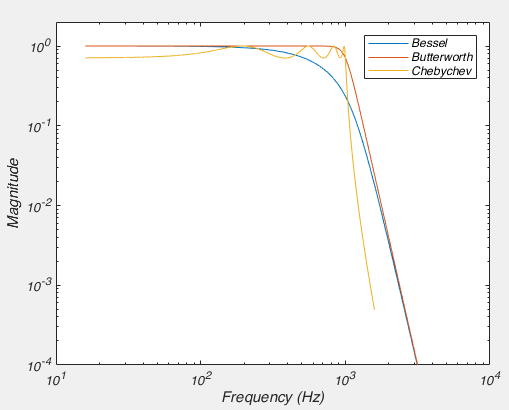
Fig 6. Frequency Response of filters of various types.
%All our filters will have a corner
%frequence (fc) of 1000 Hz
fc = 1000; % Corner Frequency of
n_poles = 8;

[zbess, pbess, kbess] = besself(n_poles, 2*pi*fc); %Create 8 pole Bessel
[bbess,abess] = zp2tf(zbess,pbess,kbess);          %Convert to transfer function
[hbess,freqbess] = freqs(bbess,abess,4096);        %Calculate Frequency Response

[bbut,abut] = butter(n_poles,2*pi*fc,'s'); %Create a 8 butterworth filter
[hbut,freqbut] = freqs(bbut,abut,4096);         %Calculate Frequency Response

[bcheb,acheb] = cheby1(n_poles,3,2*pi*fc,'s'); %Create 8 pole Chebychev   cheby1(n,3,2*pi*f,'s');
                                                    % with 3dB of ripple
[hcheb,freqcheb] = freqs(bcheb,acheb,4096);         %Calculate Frequency Response

%Plot frequency response
figure;
loglog(freqbess/(2*pi), abs(hbess))
hold on
loglog(freqbut/(2*pi),abs(hbut));
loglog(freqcheb/(2*pi),abs(hcheb));
xlabel('Frequency (Hz)');
ylabel('Magnitude');
legend('Bessel', 'Butterworth', 'Chebychev')
xlim([10 10000])
ylim([10^-4 2])
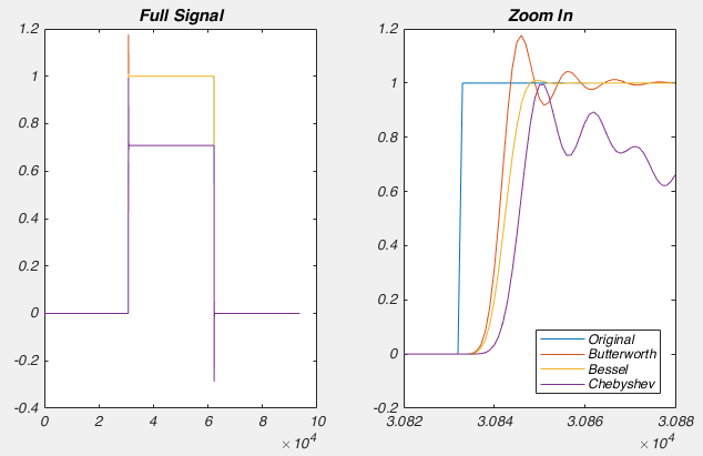
Fig 7. Different types of filters in the time domain.
Digitizing – The hidden filter
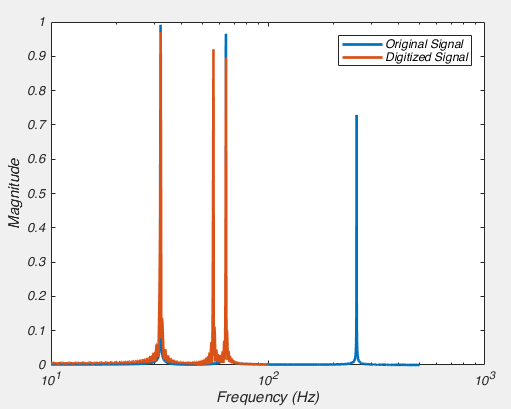
Fig 8. The affect of digitizing a signal with a 32 Hz, 64 Hz and 256 Hz component, inappropriately
%% Original, high sample rate signal
% Let us imagine this is like our analog signal

nfft = 4096;

dt = 0.001; % inter sample time = 0.001s = 1kHz sampling
t = (1:nfft)*0.001; % time vector

% Create signal vector that is the sum of 32 Hz, 64 Hz, and 256 Hz

signal = sin(32*2*pi*t) + sin(2*pi*64*t) + sin(2*pi*256*t);

f = (1/dt)/2*linspace(0,1,nfft/2+1)'; %Create Frequency vector
dft  = fft(signal, nfft)/(length(signal)/2); % take the FFT of original
mag = abs(dft(1:nfft/2+1));                  %Calculate magnitude

semilogx(f, mag, 'LineWidth', 2 );

%% Now lets digitize our faux-analog signal
% Essentially we are down sampling,
% by sampling it every 0.005s = 200 Hz = every 5th sample.

signal_dig = signal(1:5:end);
nfft_dig = 2^nextpow2(length(signal_dig)); %FFTs are faster if you perform them
                                           %on power of 2 lengths vectors


f_dig = (1/(dt*5))/2*linspace(0,1,nfft_dig/2+1)'; %Create Frequency vector
dft_dig = fft(signal_dig, nfft_dig)/(length(signal_dig)/2);
mag_dig = abs(dft_dig(1:nfft_dig/2+1));
hold on
semilogx(f_dig, mag_dig, 'LineWidth', 2);
xlim([10 1000])
xlabel('Frequency (Hz)');
ylabel('Magnitude');
legend('Original Signal', 'Digitized Signal');
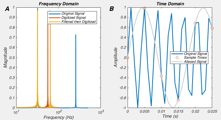
Fig 9. By filtering before we digitize, we avoid aliasing our data.
%% Let's filter the signal before we digitize it

[bbut,abut] = butter(8,100/(1000/2));      %Create a 100Hz, 8 pole butterworth filter
signal_filt = filter(bbut, abut, signal);  %Filter the data
signal_filt_dig = signal_filt(1:5:end);
dft_filt_dig = fft(signal_filt_dig, nfft_dig)/(length(signal_filt_dig)/2);
mag_filt_dig = abs(dft_filt_dig(1:nfft_dig/2+1));
semilogx(f_dig, mag_filt_dig, 'LineWidth', 2);
And this is one of the two reasons why we must ALWAYS low-pass filter data before we digitize it: if we don’t, we will get aliases, i.e. spurious frequency components. This is also what causes strange patterns in some photographs, the original data had higher frequencies (i.e. patterns changing in space) than the camera CCD could sample. The other reason we filter BEFORE was digitize is that high frequency noise can sometimes be larger than the signal we want to record, and hence filtering before digitization allows us to amplify the signal as much as possible without saturating the digitizer.
Choosing a corner and sampling frequency
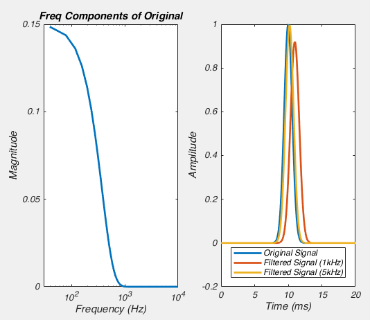
Fig 10. Trying to choose the corner frequency for a Bessel filter isn’t obvious.
dt = 1/20000; % 20kHz sampling rate
t = 0:dt:0.02; % time vector 4ms long
signal = exp(-(t-0.01).^2/(0.001/sqrt(2*log(2)))^2); %Gaussian with 1ms FWHM
nfft = 2^nextpow2(length(signal)); %FFTs are faster if you perform them
                                   %on power of 2 lengths vectors

f = (1/dt)/2*linspace(0,1,nfft/2+1)'; %Create Frequency vector
dft = fft(signal, nfft)/(length(signal)/2);      %take the FFT of original
mag = abs(dft(1:nfft/2+1));                      %Calculate magnitude

subplot(1,2,1);
semilogx(f, mag, 'LineWidth', 2);
title('Freq Components of Original')
xlabel('Frequency (Hz)');
ylabel('Magnitude');
xlim([30 10000]);
xticks([100, 1000, 10000]);

[bbess, abess] = besself(8, 2*pi*1000); %Create 8 pole 1kHz filter
[num,den] = bilinear(bbess,abess,1/dt);
signalbess1k = filter(num, den, signal); %Apply Filter

[bbess, abess] = besself(8, 2*pi*5000); %Create 8-pole 5kHz filter
[num,den] = bilinear(bbess,abess,1/dt);
signalbess5k = filter(num, den, signal); %Apply Filter

subplot(1,2,2);
plot(t*1000,signal, t*1000, signalbess1k, t*1000, signalbess5k, 'LineWidth', 2);
xlabel('Time (ms)')
ylabel('Amplitude')
legend('Original Signal', 'Filtered Signal (1kHz)', 'Filtered Signal (5kHz)', 'Location', 'south');
I should probably add that these rules of thumb are not absolute (apart from digitizing at greater than twice your filter rate: always do that!). If your filter slightly deforms the shape of your action potential, or slightly delays it in time, this may not matter for your particular experiments. But you should still be aware of the fact that if you’re filtering too close to your signal of interest, you are not recording the “true” signal.
Conclusion/Rules of Thumb
- A filter removes unwanted frequeny components
- A low-pass filter removes high frequency signals
- A filter with more poles has a steeper roll off
- A Bessel filter has the best behaviour in the time domain
- For a 4-pole Bessel, you must filter at at least 4 times the frequency of the fastest wanted component of your signal
- For an 8-pole Bessel, you must filter at at least 5 times the frequency of the fastest wanted component of your signal
- You must digitize at more than 2-3 times the frequency of your low-pass filter
Hi, I came across this while looking up how to design filters. i have a question. What if we use the “filtfilt” command instead of “filter”. Matlab documentation says that it compensates for the delay introduced by the filter.
Yes, filtfilt filters the signal first in the normal direction, going forward in time (which delays signals in time), the it takes that filtered signal and filters it again in the reverse direction, going backwards in time (which advances signals in time). This second filtering essentially undoes the time delay caused by the first filter. It also means the filter has double the number of poles of the filter you specified.
Actually, not a bad idea for a blog post seeing as how common filtfilt is just used by default.