A lot of scientists have performed Fast Fourier Transforms at some point, and those that haven’t, probably are going to in future, or at the very least, have read a paper using it. I’d used them for years before I ever began to think about how they algorithm actually worked. However, if you’ve ever looked it up, unless math is your first language, the explanation probably didn’t help you a lot. Normally you either get an explanation along the lines of “FFTs convert the signal from the time domain to the frequency domain” or you just get this:
However, the other day I came across an amazing explanation of the algorithm, and I really wanted to share it. While I might not be able to get you to the point that you completely understand the FFT, I think think it might seriously enhance your understanding.
So the first thing, I kind of lied to you. I’m not going to show you how the FFT algorithm works. I’m going to show you how discrete Fourier Transforms works. The FFT is just a fast way of computing the DFT.
So the beautiful explanation I read came from here. They color code the equation to show you how the various parts work.
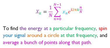
A lot of that may not be immediately obvious, though realizing that $latex e^{2 \pi i x} $ carves out a circle in the imaginary plane is a great start. The real beauty comes from the following textual explanation:
Imagine an enormous speaker, mounted on a pole, playing a repeating sound. The speaker is so large, you can see the cone move back and forth with the sound. Mark a point on the cone, and now rotate the pole. Trace the point from an above-ground view, if the resulting squiggly curve is off-center, then there is frequency corresponding the pole’s rotational frequency is represented in the sound.
There is an animation demonstrating that on the above page, but I felt a full interactive version might be helpful.
Enter in some details for two sine waves that will be summed to make your signal (graph to the left). The script will then play this waveform into our “rotating speaker” (graph to the right) which will rotate at increasing frequencies. After the waveform is played in, a red line will show up, representing a vector for the mean position of our “speaker”. The length of this vector represents the magnitude of our signal at that frequency and the angle represents the phase. The magnitude of the signal is then presented on the bottom graph, which is our DFT. Note how if you change the amplitude of your input sine waves, the length of the vector gets longer, if you change the phase, the vector points in a different direction and if you change the frequency, the vector only has a significant length when then “speaker” is rotating at that frequency. The cool thing is, while there is a lot of unnecessary graphics, the meat of this function performs a real DFT, albeit incredible slowly.
If you really want to know how FFTs work, rather than DFTs, I think this explanation is particularly good.
i never understood DFT / FFT .. coz no one explained in such a simple way.. they always said “DFT converts the signal from the time domain to the frequency domain”.. but i still wonder how & why that formula was derived… anyways.. good job keep it up!
I’ve seen that explanation before somewhere. Neat animations!
I’ve been slowly learning about Fourier series and transforms and trying to relate it to Wavelet transforms. My next step needs to be Python visualizations. Headed to matplotlib next.
Thanks for sharing!
Fast fourier transforms are an interesting mathematical approach to better understanding how sensory signals in the periphery are transduced into electrical signals used by the brain. Things like sounds waves coming into the ear are thought to use FFT models.
Nice visualization!
At engineering school (Clarkson) everyone called the FFT course “Mystery Math” cos at some point there was this instantaneous breakthru in understanding, and from that moment forward you “got it”. You just had to hope that this crucial moment came before the final exam.
I’m a 57 year old electrical engineer. I finally get it. (intuition, that is). Best. Explanation. Anywhere.
Thanks for this post, that’s a great colour-coded equation, it really helps build understanding of exactly how the DFT is computed. The youtube 3b1b has an neat video which also helps to visualuse the DFT https://www.youtube.com/watch?v=spUNpyF58BY.