In part 1 of this post, I discussed the very basics of neuronal modelling. We discussed the fundamental equations that explain how ion channels create current and how current changes the membrane potential. With that knowledge, we created a simple one-compartment model that had capacitance, and a leak ion channel. But we didn’t have any action potentials. In order to model action potentials, we need to insert some mechanism to generate them. There are several ways of doing this, but the most common is the Hodgkin and Huxley (HH) model. I’m going to dive straight in to understanding the HH model, and as usual, I’m going to start from the ground floor.
Neuronal Modelling – The very basics. Part 1.
I think a lot of people are confused about neuronal modelling. I think a lot of people think it is more complex than it is. I think too many people think you have to be a mathematical or computational wizard to understand it, and I think that leads to a lot of good modelling being discounted and a lot of bad modelling being let through peer-review. I’m here to tell you that biophysical models on neurons don’t have to be hard to implement, or understand. I’m going to start you off on the ground floor, in fact, below the ground floor, this is the basement level. All you need to know is a little coding (I’m going to do both Matlab and Python to start). But I should temper your expectations. When we are done, you’re not going to be ready to publish fully fledged multi-compartment models of neurons, but at least you will understand the fundamental principles of what is happening. And the most fundamental of all is this…
The ins and outs of field potentials
Recording field potentials was the first form of electrophysiology I ever did, and because of that, I tend to think that field potentials are simple. But the reality is far different. Field potentials, in my view, are harder to gain a solid understanding of than intracellular membrane potentials. So I’m going to try to take a ‘first principles’ approach to thinking about field potentials. To motivate us, I’m going to present exhibit ‘A’: The hippocampal CA1 population spike.
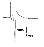
A CA1 population spike is the field potential recorded near the cell bodies of the CA1 pyramidal cells, when their afferents are stimulated strongly enough to cause the CA1 cells to spike. You see a brief upward deflection, which is an artefact from the electrical stimulation used to activate the afferents. Then you see a small downward deflection, which is due to the action potential in the afferent fibers. Then you see the population spike: the large, brief, negative potential caused by thousands of neurons spiking synchronously. It is negative because when the action potential is generated, Na+ moves into the cell, making the extracellular space negative. But here is a question: Why does the population spike appear to be resting on a positive going hump? Read on and find out, and learn more about field potentials in general.Continue reading
Freezer Monitor
We had a rash of freezers failing around the department, and I wasn’t going to become a victim. So I built something simple that has proven it’s worth. For a total cost of less than $100 you can sleep easy knowing your freezer door hasn’t been left open.
You need to understand the voltage divider!
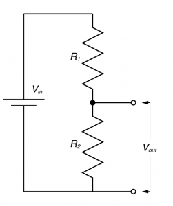
In electronic design, the voltage divider is probably the most fundamental circuit motif. You would be hard pressed to find single circuit that doesn’t have one. But more importantly, it is a deeply useful concept for explaining the physiology of excitable cells, and for understanding the nature of electrophysiological techniques. I’ve talked about voltage dividers in several of my posts, but one of my readers said I should explain what they are so that’s what I’m going to do now.
2-Photon Excitation Spectrum of Red Retrobeads
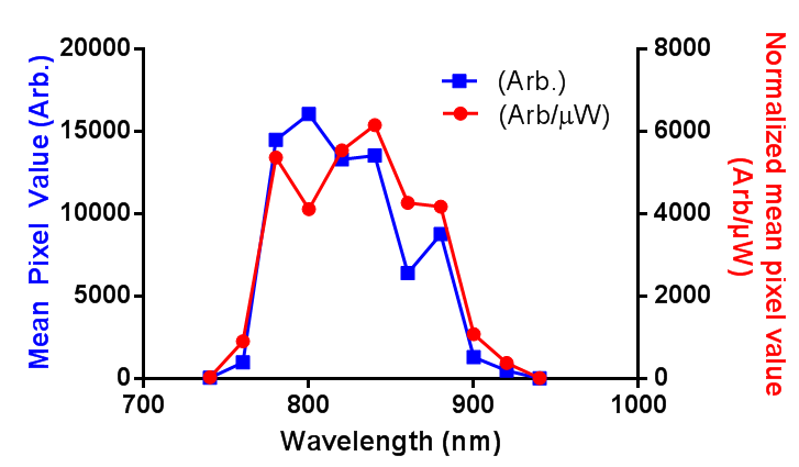
In order to successfully combined in vivo 2-photon GCaMP6f imagining and red retrobeads, I need to know the 2-photon excitation spectrum for the beads. I couldn’t find the information online, and the lumafluor didn’t have it, so I produced a rough and ready estimate. First, the power of the laser was measured in the range of 740 to 940 nm, then a small sample of undiluted retrobeads was held in the bottom of a sealed capillary tube, and the mean pixel value of the center of this capillary was measured as the wavelength was changed. I have presented the data as both the raw pixel values (Arb.) and the pixel values normalized to the power at the sample (Arb/µW). Long story short: between 780 and 880 nm is where you want to image.
EDIT: I have adjusted the axis as per the comment. I was just going to use “brightness”, but more descriptive = more better, right?
Series Resistance. Why it’s bad.
At the very start of my Masters, my first experiments appeared to show that the histamine H3 receptor inhibited the release of GABA in the neocortex. It turns out, this was all lies. It was all lies because of series resistance, a concept I had vaguely heard of, but didn’t understand. If you’re just starting electrophysiology this post is for you. The hope is that by the end of this post, you will understand series resistance, and you’ll understand why it is extremely important to monitor it religiously, whether you’re performing voltage clamp or current clamp recordings.
Continue reading
Filtering by the cell != filtering by the network
Back in 2014 I read this paper, from Judith Hirsch’s lab. To my simple mind, it was a pretty complex model, but it had a cute little video of the thalamus reducing position noise from the retina. I’m not going to lie, I still don’t fully understand the original paper, but probably due to an urge to avoid doing experiments, I felt drawn to make simple integrate and fire model of the retina -> thalamus circuit to see if it filtered noise. The result were somewhat predictable, and I tucked them away. But then an opportunity came to fish them out of the proverbial desk draw, and then I noted something quite interesting: The way the individual cells filtered their input was the opposite of how the network filtered its input. It led me to publish this article. Below you can play with some of the simulations I used to produce the paper*.
Visualizing how FFTs work.
A lot of scientists have performed Fast Fourier Transforms at some point, and those that haven’t, probably are going to in future, or at the very least, have read a paper using it. I’d used them for years before I ever began to think about how they algorithm actually worked. However, if you’ve ever looked it up, unless math is your first language, the explanation probably didn’t help you a lot. Normally you either get an explanation along the lines of “FFTs convert the signal from the time domain to the frequency domain” or you just get this:
However, the other day I came across an amazing explanation of the algorithm, and I really wanted to share it. While I might not be able to get you to the point that you completely understand the FFT, I think think it might seriously enhance your understanding.
Continue reading
Extracting data from a scatter graph
I’ve already made a rudimentary script for extracting data from published waveforms and other line graphs. But what I’ve needed recently is to be able to extract data from XY scatter graphs. This is a slightly more complex problem because it requires feature detection of an unknown number of points. You can access the script here, and I’ll go over its use and some of the code in the rest of this post. Continue reading

