In part 1 of this post, I discussed the very basics of neuronal modelling. We discussed the fundamental equations that explain how ion channels create current and how current changes the membrane potential. With that knowledge, we created a simple one-compartment model that had capacitance, and a leak ion channel. But we didn’t have any action potentials. In order to model action potentials, we need to insert some mechanism to generate them. There are several ways of doing this, but the most common is the Hodgkin and Huxley (HH) model. I’m going to dive straight in to understanding the HH model, and as usual, I’m going to start from the ground floor.

The above says that we have ion channels, and they change to ion channels with the rate constant β. The proportion of open ion channels is n, and so the proportion of closed channels must be 1-n (because all ion channels are either closed or open, and the total proportions must add up to 1). Now this reaction scheme above can be translated into the following equation:

If we remember from the last post, this means “The rate at which n changes over time is equal to -β times n”. So the more n there is, or the larger β is, the faster n decays. Why does that reaction scheme translate to that equation? Because that is what that reaction scheme means: they are just two ways of writing the same thing. Now what if we had the opposite reaction scheme, like this:

Now we are saying that the ion channels change to ion channels, with the rate constant α. Similarly, this translates to the following equation:

Which means that the rate of change of n over time (the rate at which the ion channels open) is equal to α times 1-n, or the proportion of closed channels. Hopefully you can see the pattern of how the reaction scheme turns into an equation. And hopefully, it is also making sense: in the first equation, ion channels could only go from to , so what was on the right hand side of the equation was always negative, as the amount of ion channels (i.e. n) could only decrease (because reaction rates are always positive). Likewise, in the second reaction scheme, the ion channels could only go from to , so what was on the right hand side of the equation was always positive, meaning the amount of channels was always increasing.

The last reaction scheme we need to consider is when the reaction is bidirectional, that is, ion channels can go from to and also from to . That is going to look like this:

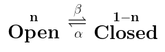
This is basically the previous two reaction schemes added together, and so the equation that explains it basically is the previous two equations added together:

If you’re still with me, we’ve done the the hard conceptual work. We just have one more problem to overcome: our rate constants α and β are not actually constant, they vary with voltage. If you’ve ever looked at a current generated during a voltage clamp family, this should make sense to you. The rate at which the current turns on depends on the voltage. Thankfully, the equations for α and β are pretty simple. For the HH potassium channel, α and β are given by

So with all that together, we can calculate what n is. But how do we go from n to a ionic current? Well I said earlier that n was the proportion of open channels. This was a lie. You should think of n as probability that a “particle” in potassium channel is in the open position. In order for the channel to conduct, you need all four of these particles to be in the open position. And just like how if the probability of getting heads in a coin flip is 0.5, then the probability of getting two heads in a row is 0.5 * 0.5, then the probability of having all four n particles in the open position is n * n * n * n or n⁴. This then tells us the proportion of potassium channels that are open, so we multiply n⁴ by the maximum possible potassium conductance, usually referred to as or “g bar”, which gives us the actual potassium conductance.

So with all of that knowledge under our belt, let’s implement this (just in python this time).

import matplotlib.pyplot as plt
import numpy as np
import math

#Functions to calculate the alpha and beta rates
#Voltage converted to mV
#Reaction rates converted to per second (Rather than per millisecond)
def alpha_n(v):
    v = v*1000
    return 0.01 * (-v-55)/( math.exp((-v-55)/10.0) -1) * 1000

def beta_n(v):
    v = v*1000
    return 0.125*math.exp((-v-65)/80.0) * 1000

# Basic simulation Properties
dt     = 10E-6;     # 10 us timestep

# Basic Cell Properties
Cm     = 100E-12;   # Membrane Capacitance = 100 pF
v_init = -70E-3;    # Initial membrane potential -70 mV

#HH Potassium Properties
n      = alpha_n(v_init)/(alpha_n(v_init)+beta_n(v_init))   # Initial condition for n

Gbar_k = 1E-6      # Maximum potassium conductance
Gleak  = 5E-9       # 5 nS conductance

Ek     = -80E-3     # Reversal for HH potassium current
Eleak  = -70E-3     # Reversal potential of -70 mV

# Injected Current step
current_magnitude = 200E-12; # 200 pA

#Injected current, 0.2 seconds of 0 current, 0.3 seconds of some current,
#and 0.5 seconds of no current
i_inj = np.concatenate( (np.zeros([round(0.2/dt),1]),
                         current_magnitude*np.ones([round(0.3/dt), 1]),
                         np.zeros([round(0.5/dt), 1])) )

#Preallocate the voltage output
v_out = np.zeros(np.size(i_inj))


#The real computational meat
for t in range(np.size(v_out)):
    if t == 1:
        v_out[t] = v_init; #At the first time step, set voltage to the initial condition
    else:
        #Calculate how the n particle changes
        dn = (alpha_n(v_out[t-1]) * (1 - n) - beta_n(v_out[t-1]) * n) * dt
        n = n + dn

        
        #Calculate the current potassium channel conductance
        Gk = Gbar_k*n*n*n*n;
        #Calculate what the current through the HH potassium channel is
        i_k = Gk * (v_out[t-1] - Ek)

        #Calculate the current through ion channels
        i_leak = Gleak * (v_out[t-1] - Eleak)  

        i_cap = i_inj[t] - i_leak - i_k   #Calculate what i is

        dv = (i_cap/Cm) * dt              #Calculate dv, using our favourite equation
        v_out[t] = v_out[t-1] + dv        #add dv on to our last known voltage

#Make the graph
t_vec = np.linspace(0, dt*np.size(v_out), np.size(v_out))
plt.plot(t_vec, v_out)
plt.xlabel('Time (s)')
plt.ylabel('Membrane Potential (V)')
plt.show()

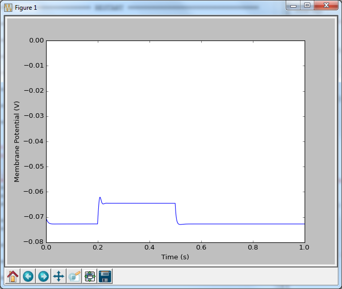Now that doesn’t look very exciting, which shouldn’t be a surprise, as we haven’t inserted any sodium channels yet. However, there are a couple things that we should go over first. On lines 8 through 14 I have two functions that calculate the alpha and beta rates. These are typically written such that mV are the units of voltage, and ms are the units of time (meaning that the reaction rates have a unit of ms^-1). I’m trying to keep everything in seconds, volts, amps etc… so I simply multiply the voltage by 1000 to get millivolts, and multiple the result by 1000 to get units of s^-1. The other thing that comes out of left field is line 24, where I set the initial condition for n. I’ve said before that when we were calculating we needed to be told what the initial conditions are, as we’re only going to add or subtract from that initial value. It’s just the same here: we need to know what n is to begin with. This equation calculates what n would be if held at the initial voltage for an infinitely long period of time, and so is a pretty good place to start. In the final post, I’m going to explain why that is, but for know, just believe me.

At line 51, we calculate what is, by following the equation I’ve already laid out, and then add it on to n. On line 56 we calculate what the current potassium conductance is, but multiplying the maximum possible potassium conductance by n⁴. Then we just follow the same equations as last time to calculate what the current is that is charging the capacitor, and then how that changes the membrane potential.

Okay, the pièce de résistance is coming: the sodium channel. Unfortunately, the sodium channel has 2 gating particles, m and h. The m particle is called the activation particle and opens when the cell is depolarized. The h particle is called the inactivation particle, and “closes” (it’s value approaches 0) when the cell is depolarized. However, when the cell is depolarized, the m particle opens faster than the h particle closes, giving you the transient nature of the sodium current. That said, the mathematics and code of these particles are essentially identical to the n particle of the potassium channel. We have alpha and beta rate constants for each particle, and they are controlled by identical functions as the n particle, just with different constants. Then the final sodium conductance is the maximum sodium conductance () multipled by m³h. So when you include them, the code looks like this:

import matplotlib.pyplot as plt
import numpy as np
import math

#Functions to calculate the alpha and beta rates
def alpha_n(v):
    v = v*1000
    return 0.01 * (-v-55)/( math.exp((-v-55)/10.0) -1) * 1000

def beta_n(v):
    v = v*1000
    return 0.125*math.exp((-v-65)/80.0) * 1000

def alpha_m(v):
    v = v*1000
    return 0.1 * (-v-40)/( math.exp((-v-40)/10.0) -1) * 1000

def beta_m(v):
    v = v*1000
    return 4*math.exp((-v-65)/18.0) * 1000

def alpha_h(v):
    v = v*1000
    return 0.07*math.exp((-v-65)/20.0) * 1000

def beta_h(v):
    v = v*1000
    return 1/( math.exp((-v-35)/10.0) +1) * 1000


# Basic simulation Properties
dt     = 10E-6;     # 10 us timestep

# Basic Cell Properties
Cm     = 100E-12;   # Membrane Capacitance = 100 pF
v_init = -80E-3;    # Initial membrane potential -80 mV

##HH Potassium Properties
# Initial condition for particles
n      = alpha_n(v_init)/(alpha_n(v_init)+beta_n(v_init))          
m      = alpha_m(v_init)/(alpha_m(v_init)+beta_m(v_init))
h      = alpha_h(v_init)/(alpha_h(v_init)+beta_h(v_init))

Gbar_k = 1E-6      # Maximum potassium conductance
Gbar_na= 7E-6      # Maximum sodium conductance
Gleak  = 5E-9      # 5 nS conductance

Ek     = -80E-3    # Reversal for HH potassium current
Ena    = 40E-3     # Reversal for HH sodium current
Eleak  = -70E-3    # Reversal potential of -60 mV

# Injected Current step
current_magnitude = 200E-12; # 200 pA

#Injected current, 0.2 seconds of 0 current, 0.3 seconds of some current,
#and 0.5 seconds of no current
i_inj = np.concatenate( (np.zeros([round(0.2/dt),1]),
                         current_magnitude*np.ones([round(0.3/dt), 1]),
                         np.zeros([round(0.5/dt), 1])) )

#Preallocate the voltage output
v_out = np.zeros(np.size(i_inj))


#The real computational meat
for t in range(np.size(v_out)):
    if t == 1:
        v_out[t] = v_init; #At the first time step, set voltage to the initial condition
    else:
        #Calculate how the particles change
        dn = (alpha_n(v_out[t-1]) * (1 - n) - beta_n(v_out[t-1]) * n) * dt
        n = n + dn

        dm = (alpha_m(v_out[t-1]) * (1 - m) - beta_m(v_out[t-1]) * m) * dt
        m = m + dm
    
        dh = (alpha_h(v_out[t-1]) * (1 - h) - beta_h(v_out[t-1]) * h) * dt
        h = h + dh
        
        #Calculate the potassium channel conductance
        Gk = Gbar_k*n*n*n*n;
        #Calculate what the current through the potassium channel is
        i_k = Gk * (v_out[t-1] - Ek)

        #Calculate the sodium channel conductance      
        Gna = Gbar_na*m*m*m*h
        #Calculate what the current through the sodium channel is
        i_na = Gna * (v_out[t-1] - Ena)

        #Calculate the current through ion channels
        i_leak = Gleak * (v_out[t-1] - Eleak)  

        #Sum all the currents
        i_cap = i_inj[t] - i_leak - i_k - i_na

        #Calculate dv, using our favourite equation
        dv = (i_cap/Cm) * dt
        #add dv on to our last known voltage
        v_out[t] = v_out[t-1] + dv      



#Make the graph
t_vec = np.linspace(0, dt*np.size(v_out), np.size(v_out))
plt.plot(t_vec, v_out)
plt.xlabel('Time (s)')
plt.ylabel('Membrane Potential (V)')
plt.show()

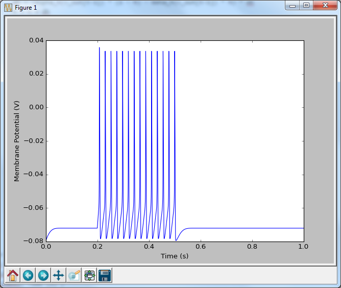And there we have it! A spiking neuron. If you read through that code, and compare it to when we just had the potassium channel, you will see that things look very similar. We are basically performing the exact same computations with slightly different alpha and beta functions. This idea extends any ion channel. Some require slightly different functions, and some may have more than one state (i.e. not just open or closed, which can get pretty complex), but the same fundamental rules apply: you set up a reaction scheme, you write the equivalent differential equation, and then you convert that to code.

In the final post, we’ll discuss a few little details I’ve skipped over, and talk about how to do this for real (spoiler: you don’t do it this way!).