Most scientists think that t-tests, ANOVAs, linear regression etc rely on your data being normally distributed. Is that really true? And given that no data is perfectly normal, how normal does your data have to be? Can I see what effect non-normality will have on my hypothesis testing? I’m going to use some simply tricks that us to see how bad our distribution is.
So I want to preface this post by saying that I don’t have a degree in biostatistics. However, this post relies on a fact that I’m pretty comfortable stating: If the null hypothesis is true (e.g. there is no difference between your populations), then P should only be less than 0.05 5% of the time. That’s half the point of null-hypothesis statistical testing! Lets write some quick python code to demonstrate this.
import numpy as np
import matplotlib.pyplot as plt
from scipy import stats

np.random.seed(1) #set random seed so you get same data
n_reps = 10000 #perform 10000 times
ps = np.zeros(n_reps)

for n in range(n_reps):
    #make two normally distributed samples, with mean=0, std dev = 1 and n = 10
    sample1 = np.random.normal(loc = 0, scale = 1, size = 10)
    sample2 = np.random.normal(loc = 0, scale = 1, size = 10)

    #perform t test
    (t, ps[n]) = stats.ttest_ind(sample1, sample2)

weights = np.ones_like(ps)/float(len(ps))

plt.hist(ps, bins = 20, weights = weights)
plt.xlabel('P Value')
plt.ylabel('Probability')
plt.title('P < 0.05 ' + str(np.sum(ps<0.05)/float(len(ps))*100) + '% of the time')
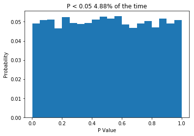
When the null hypothesis is true, P should be less than 0.05 about 5% of the time.
So what we do is create two normally distributed random variables, which have the same mean, the same standard deviation and n = 10, we subject them to a t-test, and we repeat this 10,000 times. Because the two samples are drawn from the same distribution, we would expect no difference between them, and the P values we get support that idea: getting P values less than 0.05 are relatively rare. In fact, the P value is less than 0.05 about 5% of the time, which is what leads people to say (incorrectly) that “if we reject the null hypothesis when P < 0.05, then we will only be wrong 5% of the time”. The important thing is that when testing samples where you know the null hypothesis is true, the P value should be uniformly distributed. If that is not the case, something is wrong. So what about when the null hypothesis isn’t true? Let’s change the code a little and see.
np.random.seed(1) #set random seed so you get same data
n_reps = 10000 #perform 10000 times
ps = np.zeros(n_reps)


for n in range(n_reps):
    #make two normally distributed samples, with mean=0 or 1, std dev = 1 and n = 10
    sample1 = np.random.normal(loc = 0, scale = 1, size = 10)
    sample2 = np.random.normal(loc = 1, scale = 1, size = 10)

    #perform t test
    (t, ps[n]) = stats.ttest_ind(sample1, sample2)


fig, ax = plt.subplots(1, 2, figsize=(10,4))

weights = np.ones(10000)/float(10000)
ax[0].hist(np.random.normal(loc = 0, scale = 1, size = 10000), bins = 50, weights = weights, alpha = 0.5)
ax[0].hist(np.random.normal(loc = 1, scale = 1, size = 10000), bins = 50, weights = weights, alpha = 0.5)
ax[0].set_xlabel('Sample value')
ax[0].set_ylabel('Probability')
ax[0].set_title('Sample Distributions')

weights = np.ones_like(ps)/float(len(ps))
ax[1].hist(ps, bins = 20, weights = weights)
ax[1].set_xlabel('P Value')
ax[1].set_ylabel('Probability')
ax[1].set_title('P < 0.05 ' + str(round(np.sum(ps<0.05)/float(len(ps))*100,2)) + '% of the time')
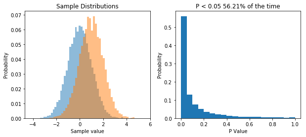
When the null hypothesis isn’t true, the distribution of P values is skewed.
So now we repeatedly perform a t-test on two samples drawn from two different populations. What we see is that now the distribution of P values is skewed, and P is less than 0.05 about 56% of the time, meaning that we have a power of 56% to detect the difference between the two populations given our sample size.
The point I want to get across is that the distribution of P values is uniform when the null hypothesis is true, and it’s skewed when the null hypothesis is false.
So now what happens if our data isn’t drawn from a normal distribution? Well let’s change our code again and see.
import numpy as np
import matplotlib.pyplot as plt
from scipy import stats

np.random.seed(1) #set random seed so you get same data
n_reps = 10000 #perform 10000 times
ps = np.zeros(n_reps)


for n in range(n_reps):
    #make two log normally distributed samples from the same population.
    sample1 = np.random.lognormal(mean = 2, sigma = 1.5, size = 10)
    sample2 = np.random.lognormal(mean = 2, sigma = 1.5, size = 10)

    #perform t test
    (t, ps[n]) = stats.ttest_ind(sample1, sample2)


fig, ax = plt.subplots(1, 2, figsize=(10,4))

#plot the distribution out data was sampled from
ax[0].hist(np.random.lognormal(mean = 2, sigma = 1.5, size = 1000), bins = 50)
ax[0].set_xlabel('Sample value')
ax[0].set_ylabel('Frequency')
ax[0].set_title('Sample Distribution')

weights = np.ones_like(ps)/float(len(ps))
ax[1].hist(ps, bins = 20, weights = weights)
plt.xlabel('P Value')
plt.ylabel('Probability')
plt.title('P < 0.05 ' + str(np.sum(ps<0.05)/float(len(ps))*100) + '% of the time')
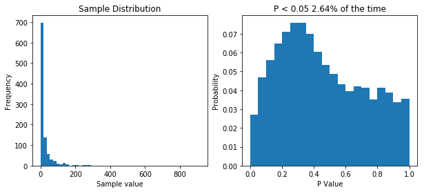
With lognormal data, our P values take on an odd distribution.
So now our samples are drawn from a lognormal distribution with a heavy positive skew. When we perform 10,000 t-tests we see that our distribution of P values is no longer uniform. This tells us that something isn’t right. But does it means we’re more likely to make type I error (rejecting the null hypothesis when we shouldn’t/false positive) or a type II error (accepting the null hypothesis when we shouldn’t/false positive). Well our simulation tested a case where the null hypothesis was true (i.e. there was no difference) and we would reject the null hypothesis when P is less than 0.05. Now P is less than 0.05 about 2.5% of the time, so our type I error rate has actually gone down. But what about the type II error rate? Well we need to run another simulation to see.
np.random.seed(1) #set random seed so you get same data
n_reps = 10000 #perform 10000 times
norm_ps = np.zeros(n_reps)
log_ps = np.zeros(n_reps)

mean1 = 1
mean2 = 2
variance = 1

for n in range(n_reps):
    #make two normally distributed samples, with mean=0, std dev = 1 and n = 10
    norm_sample1 = np.random.normal(loc = mean1, scale = np.sqrt(variance), size = 10)
    norm_sample2 = np.random.normal(loc = mean2, scale = np.sqrt(variance), size = 10)

    log_sample1 = np.random.lognormal(mean = np.log(mean1/np.sqrt(1+variance/mean1**2)), sigma = np.sqrt(np.log(1+variance/mean1**2)), size = 10)
    log_sample2 = np.random.lognormal(mean = np.log(mean2/np.sqrt(1+variance/mean2**2)), sigma = np.sqrt(np.log(1+variance/mean2**2)), size = 10)

    #perform t test
    (t, norm_ps[n]) = stats.ttest_ind(norm_sample1, norm_sample2)
    (t, log_ps[n]) = stats.ttest_ind(log_sample1, log_sample2)


fig, ax = plt.subplots(2, 2, figsize=(10,10))

weights = np.ones(10000)/float(10000)
ax[0,0].hist(np.random.normal(loc = 0, scale = 1, size = 10000), bins = 50, weights = weights, alpha = 0.5, label="Sample1")
ax[0,0].hist(np.random.normal(loc = 1, scale = 1, size = 10000), bins = 50, weights = weights, alpha = 0.5, label="Sample2")
ax[0,0].legend(prop={'size': 10})
ax[0,0].set_xlabel('Sample value')
ax[0,0].set_ylabel('Probability')
ax[0,0].set_title('Normal Population Distributions')

weights = np.ones_like(norm_ps)/float(len(norm_ps))
ax[0,1].hist(norm_ps, bins = 20, weights = weights)
ax[0,1].set_xlabel('P Value')
ax[0,1].set_ylabel('Probability')
ax[0,1].set_title('P < 0.05 ' + str(round(np.sum(norm_ps<0.05)/float(len(norm_ps))*100,2)) + '% of the time')


weights = np.ones(10000)/float(10000)
ax[1,0].hist(np.random.lognormal(mean = np.log(mean1/np.sqrt(1+variance/mean1**2)), sigma = np.sqrt(np.log(1+variance/mean1**2)), size = 10000), weights = weights, alpha = 0.5, bins = np.linspace(0,20,100), label="Sample1")
ax[1,0].hist(np.random.lognormal(mean = np.log(mean2/np.sqrt(1+variance/mean2**2)), sigma = np.sqrt(np.log(1+variance/mean2**2)), size = 10000), weights = weights, alpha = 0.5, bins = np.linspace(0,20,100), label="Sample2")
ax[1,0].legend(prop={'size': 10})
ax[1,0].set_xlabel('Sample value')
ax[1,0].set_ylabel('Probability')
ax[1,0].set_title('Lognormal Population Distributions')

weights = np.ones_like(log_ps)/float(len(log_ps))
ax[1,1].hist(log_ps, bins = 20, weights = weights)
ax[1,1].set_xlabel('P Value')
ax[1,1].set_ylabel('Probability')
ax[1,1].set_title('P < 0.05 ' + str(round(np.sum(log_ps<0.05)/float(len(log_ps))*100,2)) + '% of the time')
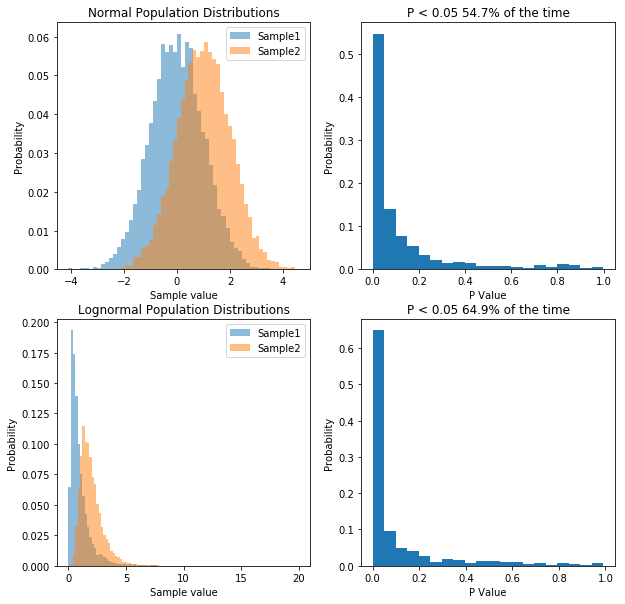
Lognormal distributions INCREASE our power? Not really
So what we’ve done is run 10,000 simulations of two experiments. In one we take samples from two normal populations, both with a standard deviation of 1, and means of 1 and 2 respectively. In the other, we take samples from two lognormal populations, again, with a standard deviation of 1, and means of 1 and 2 respectively. As before, when we sample from a normal distribution, our t-test has a power of about 55%. However, in the case of our lognormal distribution we end up with a power of 65%. So does that mean people have been lying to you, and that doing statistics on non-normal data is actually better?. That would be the wrong conclusion, because if we transform the data, we can get even higher power. Specifically, if we log our lognormal data, and make it normally distributed, our power goes up significantly. Check it out:
np.random.seed(1) #set random seed so you get same data
n_reps = 1000 #perform 10000 times
norm_ps = np.zeros(n_reps)
log_ps = np.zeros(n_reps)

mean1 = 1
mean2 = 2
variance = 1

for n in range(n_reps):
    log_sample1 = np.log(np.random.lognormal(mean = np.log(mean1/np.sqrt(1+variance/mean1**2)), sigma = np.sqrt(np.log(1+variance/mean1**2)), size = 10))
    log_sample2 = np.log(np.random.lognormal(mean = np.log(mean2/np.sqrt(1+variance/mean2**2)), sigma = np.sqrt(np.log(1+variance/mean2**2)), size = 10))

    #perform t test
    (t, log_ps[n]) = stats.ttest_ind(log_sample1, log_sample2, equal_var=False)


fig, ax = plt.subplots(1, 2, figsize=(10,4))

weights = np.ones(10000)/float(10000)
ax[0].hist(np.log(np.random.lognormal(mean = np.log(mean1/np.sqrt(1+variance/mean1**2)), sigma = np.sqrt(np.log(1+variance/mean1**2)), size = 10000)), weights = weights, alpha = 0.5, bins = np.linspace(-4,4,100), label="Sample1")
ax[0].hist(np.log(np.random.lognormal(mean = np.log(mean2/np.sqrt(1+variance/mean2**2)), sigma = np.sqrt(np.log(1+variance/mean2**2)), size = 10000)), weights = weights, alpha = 0.5, bins = np.linspace(-4,4,100), label="Sample2")
ax[0].legend(prop={'size': 10})
ax[0].set_xlabel('Sample value')
ax[0].set_ylabel('Probability')
ax[0].set_title('Log(Lognormal Population Distributions)')

weights = np.ones_like(log_ps)/float(len(log_ps))
ax[1].hist(log_ps, bins = 20, weights = weights)
ax[1].set_xlabel('P Value')
ax[1].set_ylabel('Probability')
ax[1].set_title('P < 0.05 ' + str(round(np.sum(log_ps<0.05)/float(len(log_ps))*100,2)) + '% of the time')
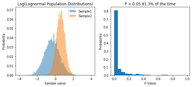
Transforming the data to make it normal maximizes your power.
So transforming the data to make it normal has increased our power. So basically, working with lognormal data decreases our type I error rate, but INCREASES our type II error rate, relative to normal data.
Okay, so now we know how to see what kind of effect sampling simulated data from perfect distributions has on our statistics. But can we look at our own data and get an idea of how much of an effect it’s non-normality will have on our results? Normality tests like the Anderson-Darling test aren’t much use here. If your sample size is small, normality tests will nearly always tell you you data is normal, and if your sample size is large, even negligible deviations from normality will cause the test to tell you that your data is not normal. In reality, we don’t want a test to tell you whether your data is exactly, perfectly normal. You want to know whether its deviations from normality matter. So what we can do instead is generate a simulated population that matches our data, then draw random samples from it. Thankfully this is actually pretty easy to in python, though it does require a bit of care.
import numpy as np
import matplotlib.pyplot as plt
from sklearn.neighbors import KernelDensity

data = np.array([0.9390851, 0.9666265, 0.7483506, 0.9564947, 0.243594, 0.9384128, 0.3984024, 0.5806361, 0.9077033, 0.9272811, 0.9013306, 0.9253298, 0.9048479, 0.9450448, 0.8598598, 0.8911161, 0.8828563,0.9820026,0.9097131,0.9449918,0.9246619,0.9933545,0.8525506,0.791416,0.8806227,0.8839348,0.8120107,0.6639317,0.9337438,0.9624416,0.9370267,0.9568143,0.9711389,0.9332489,0.9356305,0.9160964,0.6688652,0.9664063,0.4913768]).reshape(-1,1)
x = np.linspace(-1, 2, 100).reshape(-1,1)


fig, ax = plt.subplots(1,3, figsize=(10,4), sharey=True)
bw = [0.25, 0.05, 0.01]
ax[0].set_ylabel('Normalized PDF')
for n in range(ax.size):
    #Create our estimated distribution
    kde = KernelDensity(kernel='gaussian', bandwidth=bw[n]).fit(data)

    #Plot our estimated distribution
    plt.sca(ax[n])
    ax[n].fill(x, np.exp(kde.score_samples(x))/np.max(np.exp(kde.score_samples(x))), '#1f77b4')
    ax[n].plot(data, np.random.normal(loc = -0.05, scale = 0.01, size= data.size), '+k')
    ax[n].set_xlim(-0.5, 1.5)
    plt.xticks([0, 1])
    ax[n].set_ylim(-0.1, 1.1)
    ax[n].set_title('Bandwidth = '+str(bw[n]))
    ax[n].set_xlabel('Sample value')
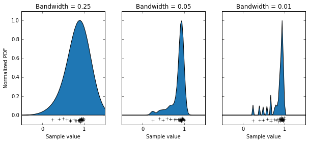
Modelling distributions requires a careful choice of parameters.
What we’ve done is use the KernelDensity function from the scikitlearn package, which generates a probability density function by summing up lots of little functions AKA a kernel, where each data point is. The choice of an appropriate kernel is key to generating a good probability density function. In this case we’ve chosen a Gaussian kernel, but we can still alter it’s “bandwidth” (basically it’s standard deviation). I have some data that is the orientation selectivity index of some axon terminals (the data points along the bottoms of the graphs). This measure can only take on values between 0 and 1. We can see that using a bandwidth of 0.25 has done a bad job of modelling our population, as it’s saying values above 1 are quite likely, and that the distribution is basically symmetrical. Using a bandwidth of 0.01 has also done a bit of a bad job, as you can see it’s made a multi-modal distribution, which I’m pretty sure isn’t accurate. Using a bandwidth of 0.05 seems to have done a pretty good job, producing a relatively smooth curve which seems to model out data well. So with that decided, let’s use that probability density function to sample some data, and do some t-tests when the null hypothesis is true
import numpy as np
import matplotlib.pyplot as plt
from scipy import stats
from sklearn.neighbors import KernelDensity

np.random.seed(1) #set random seed so you get same data
n_reps = 10000 #perform 10000 times
ps = np.zeros(n_reps)

data = np.array([0.9390851, 0.9666265, 0.7483506, 0.9564947, 0.243594, 0.9384128, 0.3984024, 0.5806361, 0.9077033, 0.9272811, 0.9013306, 0.9253298, 0.9048479, 0.9450448, 0.8598598, 0.8911161, 0.8828563,0.9820026,0.9097131,0.9449918,0.9246619,0.9933545,0.8525506,0.791416,0.8806227,0.8839348,0.8120107,0.6639317,0.9337438,0.9624416,0.9370267,0.9568143,0.9711389,0.9332489,0.9356305,0.9160964,0.6688652,0.9664063,0.4913768]).reshape(-1,1)
x = np.linspace(-1, 2, 100).reshape(-1,1)

kde = KernelDensity(kernel='gaussian', bandwidth=0.05).fit(data)

for n in range(n_reps):
    sample1 = kde.sample(10)
    sample2 = kde.sample(10)
    (t, ps[n]) = stats.ttest_ind(sample1, sample2)


fig, ax = plt.subplots(1, 2, figsize=(10,4))

#plot the distribution out data was sampled from
weights = np.ones(10000)/float(10000)
ax[0].hist(kde.sample(10000), bins = 50, weights = weights)
ax[0].set_xlabel('Sample value')
ax[0].set_ylabel('Probability')
ax[0].set_title('Population Distribution')

weights = np.ones_like(ps)/float(len(ps))
ax[1].hist(ps, bins = 20, weights = weights)
plt.xlabel('P Value')
plt.ylabel('Probability')
plt.title('P < 0.05 ' + str(np.sum(ps<0.05)/float(len(ps))*100) + '% of the time')
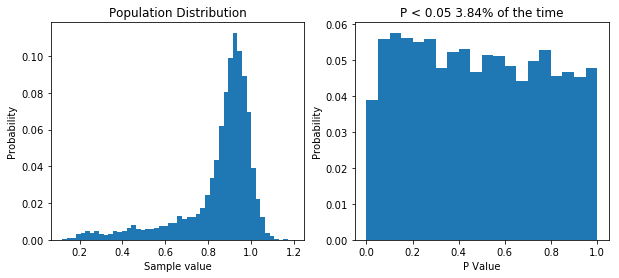
Simulating our non-normal data allows us to show that we’d almost half our type I error rate if we used it.
So like when we were dealing with non-normal data before, our type I error rate has gone down. So you can bet our type II error rate is higher than it needs to be. But let’s prove it. First, I think that transforming our data by taking a large number, say 100, and raising it to the power of our data will make the data more normal. If that’s true, out P value distribution in the null case should be more uniform, and the power in the non-null case should be higher. I’ll spare you the code, though it’s available here. But the result is what I predicted, as you can see below.
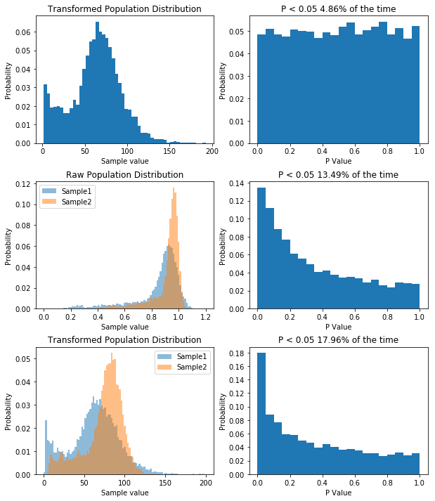
Even a pretty rough transform improves things
So by applying our transform we’ve seen how having non-normal data decreases our type I error rate, but increases our type II error rate. For what it’s worth, with the kind of data I had, trying to transform it to normality was a bad idea, as it will never become normal, and I’d be better off using a different model altogether, but the underlying concept remains: you can use KernelDensity to allow you to draw data from your own distribution.
Finally, there is one more thing I want to cover. Some statisticians like to point out that when performing good old fashioned t-tests and ANOVAs, there is no assumption of normality: the data can follow any distribution and hypothesis testing will be legitimate. In certain cases, this is true. Specifically, if the sample size is big enough, even wildly non-normal data will behave well in parametric tests. However, even with relatively tame non-normal data, the number of samples require before the t-test is well behaved can be very large, well outside the range that most physiologists will be able to achieve. The figure below shows that. I’ve done what I’ve done before and performed 10,000 t-tests on data from the same population, with varying sample sizes. Even with a sample size of 100, the distribution of p values isn’t uniform.
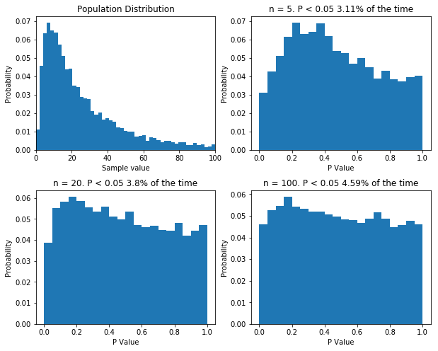
If your sample size is large enough, classical null-hypothesis statistical testing is well behaved with non-normal data. But the sample size might need to be very large. Even with n = 100, the distribution of p values in the null case is not uniform.
I should point out that there are a bunch of caveats here. For instance, if you’re the first person to measure something, and you have n = 5, then you probably can’t usefully use KernelDensity to construct a population distribution, as you have no idea what it looks like. For much the same reason, you can’t use the techniques I’ve demonstrated to measure the power of your hypothesis testing based on your samples: power analysis relies on know population variables, not sample variables… There are probably other caveats, I’ll let you know once people on twitter tell me.
So in conclusion, if hypothesis testing is working properly, when the null hypothesis is true, P values should be uniformly distribution. If the null hypothesis is not true the distribution of P values is skewed. For P values to mean what you think they mean, when you perform standard t-tests and ANOVAs your data needs to be normally distributed unless you have very large sample size. With a bit of care you can use KernelDensity to simulate your population of interest. Then you can perform t-tests on the null-hypothesis to simply look at your type I error rate. And so long as you have a way of transforming your data to make it normal, you can then see what effect doing analysis on your untransformed data has on your type II error rate. Often you don’t know how to transform your data to make it normal and that is why simulating the null hypothesis is so useful.