It seems like every paper I look at these days has Nonnegative Matrix Factorization (NMF) in its methods somewhere. From machine learning, to calcium imaging, the seemingly magic ability of NMF to pull apart signals gets a lot of use. In this post I want to explain NMF to people who have zero understanding of linear algebra, show a few applications, and maybe give you some inspiration of how to use NMF in your own work.

So Nonnegative Matrix Factorization (NMF) can be explained in a variety of ways, but I think the simplest way is that NMF reveals your signal’s component parts. That is to say, if your signal is the sum of a variety of other signals, then NMF will reveal those underlying signals. To me, this naturally makes me think of signals that vary over time, but NMF can be used on a variety of other signals, like images, or text. However, in order to get to the examples, we need to understand how NMF works. So lets break NMF down, word by word. (If you’re fine with the concepts of matrix multiplication and factorization, skip down to “Example 1 – Time series“).

Nonnegative

This is the easiest bit to explain. NMF only works on signals that are always positive. I’ve said that NMF splits a signal up into the individual elements that are summed up to make the signal. Because the signal must always be positive, the individual elements must also be positive. However, you can take a negative signal, add some positive value to it and it becomes positive. So then you can use NMF on it, right? Well not always. What is more important to think about is the individual elements. To make your signal, are the individual elements always added together, or is one element subtracted from another? If it is the former, then NMF may work, even if the signal is always negative (once you add a constant to the data to make it positive). If it is the later, NMF will never work. For example, lets say we were interested in the amount of a contaminant in lake. Every day various factories dumped discharge into the lake. Perhaps we could use NMF to figure out how each factory affected the amount of contaminant in the lake (because the total contaminant is a sum of all the discharges from each factory). However, if the lake was sometimes cleaned of the contaminant, NMF probably isn’t appropriate, as we now have a subtractive signal mixed in with our additive signal.

Matrix

Even the word “matrix” may intimidate some people. There is nothing magical about matrices. They are just a collection of numbers arranged in a square/rectangle. And just like there are rules for how you multiply numbers, there are rules for how you multiply matrices, rules that you need to understand in order to understand NMF. While these rules may seem a little weird if you’re only used to multiplying numbers, thankfully, they’re not very difficult to remember. It’s easiest to just see the rules in action. Concretely, if we have two matrices, X and Y where:

Then we calculate X × Y by doing the following

So if we look at element a in the product matrix X × Y (i.e. the number in first column, first row), we see it is somehow related to the first row of matrix X, and the first column of matrix Y. We see that the first element in the first row of matrix X is multiplied by the first element in the first column of matrix Y, and this is added to the product of the second element in the first row of matrix X and the second element in the first column of matrix Y. It’s worth noting at this point that this means that X × Y produces a matrix that is NOT the same as Y × X.

If you’ve never come across matrix multiplication before, this may all seem very strange, very pointless and very annoying. But let me show one way of thinking of matrix multiplication that hopefully will make it make some sense, or at least give it some utility. Let us say that matrix X is some data, we can then see matrix Y and set of weights, where X × Y is now a sort of weighted average of X. How does this work? Well, if the first row of X is a set of obervations, then the first column of Y is our weights. As we move across the elements in that row of X (our data), we look to the corresponding element in the column of Y (our weights), and multiply the two together. If the element in Y is large, then that element of X is amplified. If the element in Y is zero, then that element of X is ignored. But lets look at a concrete example. We have matrices X and Y,

and we multiply them together:

Because the first element of the first column of Y is 1, we then apply this weighting to the first element of the first row of X. However, the second element of the first column of Y is zero. This means we apply a zero weight to second element of the first row of X. We sum these two products (3 × 1 + 1 × 0 = 3) and we put the result in the first row, first column of X × Y. When we go down to the second row of X, we again apply the weights of the first column of Y, and the element in the second row, first column of X × Y is 2 × 1 + 5 × 0 = 2. Notice, because the first column of Y was [1 0] now the first column of X × Y is [3 2], i.e. we applied a weighting of 1 to the first column of X, and a weighting of zero to the second column, and so we just reproduced first column of X. In order to calculate what will be in the second column of X × Y, we apply the weights see in the second column of Y, to the data in X.

So to put this really succinctly, the element in the ith row, jth column of the matrix X × Y is the data in the ith row of X, weighted by the weights in the jth column of Y. If any element, say element n, in the jth column of Y is much much larger than all the other elements in that column, then then jth column of X × Y will essentially be equal to the nth column of X, multiplied by the value of that nth element in Y. I’m going restate that idea again, because it is super important later on: As we travel down a column in Y, if any element is much much larger than all the others, then that same column of X × Y will be essentially equal to the equivalent column of X, multiplied by a constant.

This may all be a lot to take in, so as hopefully a simple exercise that will help you see how when you calculate X × Y, Y acts like a set of weights. What is the product of these two matrices:

Factorization

Hopefully you haven’t completely forgotten high school math, but if you have, factorization is solving this problem: if we have a number a, what are all the values of x and y such that x × y = a. So, the factors of the number 4 are 1, 4 and 2, as 1 × 4 = 4, and 2 × 2 = 4. These are strictly speaking, the positive integer factors of 4. There are an infinite number of non-integer factors, e.g. 0.25 × 16 = 4, -0.1 × -40 = 4 etc… We can factor matrices just the same. The factors of matrix Z are all the matrices such that X and Y such that X × Y = Z. And just like factorizing numbers, there can be a large number of factors for a given matrix, even an infinite number. But if you’re new to matrices there is a reason that there can be a large number factors for a given matrix that might not be immediately obvious: size.

If our matrix Z is 2 x 2 matrix, what sizes can the factors of Z be? Well any size, so long as X has 2 rows, and Y has 2 columns, and the “inner dimension” of X and Y match (“inner dimension” is the number of columns X has and the number of rows Y has) there may be factors of any size, see:

Matrix factorization (sometimes called “decomposition”) is a complex field, there are tonnes of approaches to factor matrices, with different goals and applications, but the different ways of factorizing a matrix all do fundamentally the same thing, you give it a matrix, and it gives you two (or more) matrices, that when multiplied together give you your original matrix or close approximation to it.

Approximation? How can you say two matrices are a factor of another matrix if it is only an approximation? Well it turns out a) factoring matrices is often very computationally complex b) some matrices don’t even have factors, especially given constraints like nonnegativity and c) an approximation is often good enough.

Alright, enough background, let’s get into how this works.

Example 1 – Time series

So earlier I gave a made up example: There are 3 factories that dump contaminants into a lake. Whether the factory dumps each day is random (so not all factories are active every day, in fact, if all factories were active every day, we couldn’t tease apart their signals). Each factory dumps a different amount of the contaminant with a different time course. We measure the concentration of the contaminant in the lake. We collect data for 1000 days. Can we figure out what each factories outflow looks like? With NMF we can.

First lets simulate our data:

rng(0);

%The output of each factory
factory1 = [0; 0; 9; 5; 3; 2; 1; 0; 0; 0; 0; 0];
factory2 = [0; 0; 0; 0; 0; 3; 2; 1; 1; 0; 0; 0];
factory3 = [0; 5; 5; 6; 6; 7; 4; 2; 1; 0.5; 0; 0];

%a matrix to store the all, for ease later on.
allfactories = horzcat(factory1, factory2, factory3);

num_days = 1000; % we collect data for 100 days

data = zeros(12,num_days); % preallocate matrix to store our data

h = figure();
set(h, 'MenuBar', 'none');
set(h, 'ToolBar', 'none');
subplot(2,1,1);
plot(allfactories);
xlabel('Time (hours)');
ylabel('Factory output');
legend('Factory 1', 'Factory 2', 'Factory 3');
title('Individual Factories')

for d = 1:num_days
   which_factories = boolean(randi([0 1], 1, 3)); %Randomly decide which factory discharges today
   output_for_day = sum(allfactories(:, which_factories), 2); %sum the output of active factories
   data(:,d) = output_for_day;   
end

subplot(2,1,2);
plot(output_for_day);
hold on;
plot(allfactories(:, which_factories), '--', 'Color', [0.5 0.5 0.5]);
hold off
xlabel('Time (hours)');
ylabel('Amount in lake');
legend('Total Output', 'Individual Output');
title('Data from day 1000')

Which should make a figure like this, where on the top we have the output of each factory, and on the bottom we have the concentration of contaminant in the lake on an arbitrary day, and how each factory contributed (only two factories dumped that day).

Now we’re going to do our NMF. It’s VERY important to think about this carefully. We need to lay our data out right, or the output of your NMF will be garbage. Specifically, each column of our data matrix needs to be a single observation, while each row of our matrix is the same data from a different observation. So in our example, each column is data from a different day, and each row is a different hour.

Why this is so crucial is that we can only understand the matrix factorization if we understand the data. Specifically, if we organize the data in this way, then when we factorize our data matrix such that W × H = Data, then the columns of W make up our signals that sum to make our data, and H make up our weights (in NMF, the factors are always called W and H, and I don’t know why). Have a look at this figure, and maybe re-read the section on matrix multiplication if you don’t see why.

Running NMF is simply a one line command in MATLAB.

[W, H] = nnmf(data, 3, 'replicates', 100);

Let’s just go over the one line in detail, we are saying we want to perform NMF on the matrix data, and return the factors W and H. The second argument 3 is stating how many individual signals we are trying to break the data down into. In our example, we know there are three factories. So we know 3 is a good number. Sometimes in real life, you wont know what value to use here, and it’s beyond the scope of this article to talk about how to choose values. The second and third argument is a parameter-value pair, where I am telling the algorithm to perform the factorization 100 times, and then choose the best one. This can be important. NMF is solved numerically, with the computer first having a random guess at the solution, and then iteratively improving it. Depending on that first guess, the final solution can vary significantly. Hence it is important to have many initial guesses and only choose the best solution.

So we run that line and what do we expect? W×H should equal our data, H should be a matrix filled with 0s and 1s, and the matrix W should be identical to our matrix allfactories. Why? Well W×H should equal our data because that is the whole point of NMF: finding two matrices that when multiplied together make our data. We expect H to be full of 0s and 1s, because those are the weights which say on a given day (column) which factories were dumping. Finally, we expect W to be equal to allfactories, as allfactories is a matrix containing the possible outputs of each factory, i.e. the individual signals that make up our data.

So what do we see? Well it certainly seems like W×H very closely approximates our data:

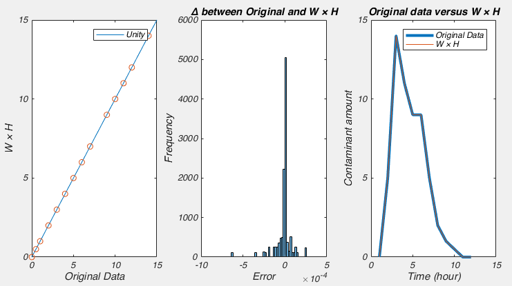
But matrix H is not full of 0s and 1s. It seems to be full of numbers close to 0 and numbers around 0.045. This is because there are many ways to factor a number, i.e. 0.5 × 8 = 4, just like 2 × 2 does. And in this case, the NMF algorithm had no idea that we expected matrix H to be 0s and 1s, so it did the best it could. For a similar reason, the values in matrix W seem too large. However, this is easy to fix: we simply scale matrix H by dividing it by its maximum value, and scale matrix W by multiplying it by the same value. And lo and behold, the columns of W now contain the estimate of the output of each factory and columns of H tells us on which days each factory dumped.

 max(H(:))

ans =

    0.0507
% This isn't good

scale_factor = max(H(:));
H = H./scale_factor;
W = W.*scale_factor;

h3 = figure();
set(h3, 'MenuBar', 'none');
set(h3, 'ToolBar', 'none');

plot(W, 'Color', [0.4 0.4 0.7], 'LineWidth', 2)
hold on
plot(allfactories, 'Color', [0.7 0.4 0.4], 'LineWidth', 2)
xlabel('Time (hour)')
ylabel('Contaminant amount')
legend('Original Factory Ouput','','', 'NMF Approximation','','');

You can see that the approximation isn’t perfect, we could improve that possibly by running the nnmf() function with more replicates, by allowing it more iterations before it terminates and certainly by collecting more data. But nonetheless, I hope you see the importance of what has just happened, with nothing more than the raw data, an assumption that the data was a sum of positive signals, and the knowledge of how many signals there are, NMF has almost perfectly pulled apart those signals.

Example 2 – Calcium Imaging

I wont bore you with the code, but I made a model of some calcium imaging data, where I have 5 cells glowing, and their brightness changes over time. Like this:

Conceptually, you should be able to see how each frame of this video is basically a sum of the activity of these five cells. So we should be able to use NMF to factorize this data into a W matrix that contains a picture of each cell, and an H matrix that contains information related to how bright each cell is in time. However, there is a complication. Like any normal person would, I have stored this movie as a [height] x [width] x [number of frames] matrix, i.e. a 3D matrix. NMF only works on 2D matrices. So what do we do? Well have have to reshape our movie so that each column is one frame, and each row is a particular pixel, i.e. the first column is the first frame, and the first row is the top left pixel, like this:

Once we’ve done that, NMF should be able to factorize the matrix like this:

This may seem a bit hard to grasp at first, but go back to the factory example: there, each column of W was the output of each factory, and H told us if the factory was active or not. This is very similar, W is the “shape” of each cell, and H tells us how active that cell is. After we run NMF, we simply reshape each column of W back into a height x width matrix to see each cell, and we plot each row of H to see how active it is.

So when we run the NMF on that movie above, we can extract the following data: the images on the left are the reshaped columns of matrix W, and the graphs on the right are the rows of matrix H (again, I had to apply some scaling factor to W and H).

Now while I’m not suggesting that everyone drops their hand drawn ROIs just yet, you’ve got to admit that one line of matlab code achieving that is impressive. If you want to have a go yourself, the script is available here.

Example 3 – Faces

So now we’re going to do something weird. We’re going to try to factorize faces. You can kinda see how a face can be seen as a sum of different parts, e.g. eyes, noses, mouth. We have a dataset here called the “Frey Faces” which are 2000 images of Prof. Brendan Frey making faces at a camera.

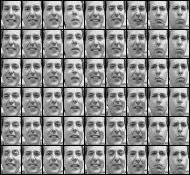
After some thought, you should be able to see that NMF is unlikely to pull out images of eyes, noses etc, because every image contains eyes, noses etc, i.e. these aren’t the individual signals that are summed to make each photo. What changes are the expressions. So what we should pull out are the signals that vary with each expression. It’s also worth pointing out that, unlike the 3 factory or 5 cell example, in this data set, we don’t know the number of individual signals. But have a quick look at the dataset, I’m going to say there are 8 primary facial expressions. Like always, we need to organize our data, in this case so that each column represents one face, and each row represents a given pixel. Running the NMF, and then reshaping the columns of W back to the right size shows us the supposed individual signals that make up the total.

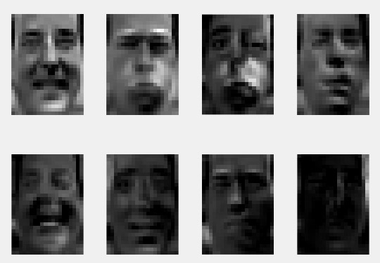
Some of these individual signals seem believable, others a little strange, but lets roughly gauge how well we did by comparing the original faces to those reconstructed when we multiply H by W.

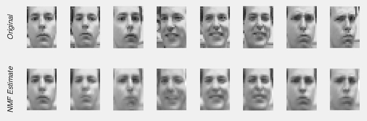
I believe it is fair to say that these are convincing, though not perfect, estimates of the original.

Obviously, there is no scientific breakthrough here. But I just wanted to show how varied applications of NMF can be.

Summary

So NMF is a technique that splits your data up into a set of individual signals and weights to apply to those signals to recreate your original data. It works best when your data is truly a sum of individual signals (e.g. the factory and calcium imaging examples) but it will still work to some degree when the data isn’t quite like that (the faces). There are some caveats when it comes to applying NMF that I have mentioned (e.g. the data needs to be positive, and laid out in an appropriate matrix) but a variety I haven’t mentioned (what is the relationship between the number of observations/columns in the data matrix and the number of individual signals you can decompose the data into?). But this wasn’t meant to be a comprehensive discussion of NMF, just something to get you started.

If you want to see some published application of NMF and to make it clear that I don’t think I’m the first person to invent the idea of using NMF to probe calcium imaging data or faces, have a look at this paper “Simultaneous Denoising, Deconvolution, and Demixing of Calcium Imaging Data” from the Paninski lab or “Learning the parts of objects by non-negative matrix factorization” from Lee & Seung.