I think a lot of people are confused about neuronal modelling. I think a lot of people think it is more complex than it is. I think too many people think you have to be a mathematical or computational wizard to understand it, and I think that leads to a lot of good modelling being discounted and a lot of bad modelling being let through peer-review. I’m here to tell you that biophysical models on neurons don’t have to be hard to implement, or understand. I’m going to start you off on the ground floor, in fact, below the ground floor, this is the basement level. All you need to know is a little coding (I’m going to do both Matlab and Python to start). But I should temper your expectations. When we are done, you’re not going to be ready to publish fully fledged multi-compartment models of neurons, but at least you will understand the fundamental principles of what is happening. And the most fundamental of all is this…

Before I get started, I just want to say, that if you know what a Jacobian Matrix is, or what Runge–Kutta methods are, this post is not for you. This is neuronal modelling for people at the back of the class.

As I said above, the most fundamental equation in all of this is this:

Which is saying “The rate at which the membrane potential changes is equal to the current flowing, divided by the capacitance of the cell”. But to make it even more clear, let’s look into the left part of the equation: which may already be scaring you. I want you to treat this as just a normal fraction, just like where the symbol just means “a little bit of” so means “a little bit of v divided by a little bit of t”, where v is voltage and t is time. So what we’re saying is, in a little bit of time, how much does v change? Because we’re treating as a simple fraction, we can just multiply each side by and get the equation

So what we are saying is: “The amount that the membrane potential changes (in a small amount of time) is equal to the current flowing, divided by the capacitance of the cell multiplied by that small amount of time. And THAT is basically what all neuronal models perform: for each compartment of the cell, it calculates what i is, then performs that computation. What you might notice is that we’re only talking about how the membrane potential changes, not what it actually is. And because of that, we need to choose where the membrane potential begins or what is called “the initial conditions”.

With that knowledge in mind, let’s convert this mathematics to code and get started with becoming computational neuroscientists.

Matlab

% Basic simulation Properties
dt     = 10E-6;     % 10 us timestep

% Basic Cell Properties
Cm     = 100E-12;   % Membrane Capacitance = 100 pF
v_init = -70E-3;    % Initial membrane potential -70 mV

% Injected Current step
current_magnitude = 100E-12; % 100 pA 

%Injected current, 0.2 seconds of 0 current, 0.3 seconds of some current,
%and 0.5 seconds of no current
i_inj = [zeros(round(0.2/dt),1);
         current_magnitude*ones(round(0.3/dt), 1);
         zeros(round(0.5/dt), 1)];

%Preallocate the voltage output
v_out = zeros(size(i_inj));

%The real computational meat
for t = 1:length(v_out)
    if t == 1
        v_out(t) = v_init; %At the first time step, set voltage to the initial condition
    else
        i_cap = i_inj(t);       %Calculate what i is
        dv = i_cap/Cm * dt;     %Calculate dv, using our favourite equation
        v_out(t) = v_out(t-1) + dv;     %add dv on to our last known voltage
    end
end

%Make the graph
t_vec = dt*[1:length(v_out)];
plot(t_vec,v_out);
xlabel('Time (s)')
ylabel('Membrane Potential (V)')

Python

import matplotlib.pyplot as plt
import numpy as np

# Basic simulation Properties
dt     = 10E-6;     # 10 us timestep

# Basic Cell Properties
Cm     = 100E-12;   # Membrane Capacitance = 100 pF
v_init = -70E-3;    # Initial membrane potential -70 mV

# Injected Current step
current_magnitude = 100E-12; # 100 pA

#Injected current, 0.2 seconds of 0 current, 0.3 seconds of some current,
#and 0.5 seconds of no current
i_inj = np.concatenate( (np.zeros([round(0.2/dt),1]),
                         current_magnitude*np.ones([round(0.3/dt), 1]),
                         np.zeros([round(0.5/dt), 1])) )

#Preallocate the voltage output
v_out = np.zeros(np.size(i_inj))

#The real computational meat
for t in range(np.size(v_out)):
    if t == 0:
        v_out[t] = v_init; #At the first time step, set voltage to the initial condition
    else:
        i_cap = i_inj[t];       #Calculate what i is
        dv = i_cap/Cm * dt;     #Calculate dv, using our favourite equation
        v_out[t] = v_out[t-1] + dv;     #add dv on to our last known voltage

#Make the graph
t_vec = np.linspace(0, 1, np.size(v_out))
plt.plot(t_vec, v_out)
plt.xlabel('Time (s)')
plt.ylabel('Membrane Potential (V)')
plt.show()

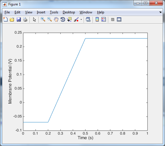Despite the length of that code, all the import stuff is happening in the for loop. At the first time point we set the voltage equal to the initial voltage, and from then on at each time point we calculate the new voltage by adding something (dv) onto the previous voltage. Now you may be looking at the voltage trace and thinking that it doesn’t look very neuronal. Well that is because we have no ion channels. In order to include ion channels, we need to know how they behave. The standard model for an ion channel starts with this simple formula:

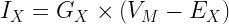
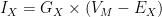
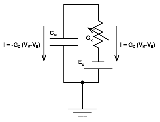Where we are saying the ionic current for an ion channel X (), is equal to the conductance of the ion channel (), multiplied by the driving force, where the driving force is the membrane potential () minus the reversal potential of that ion channel (). To include this into our model, we need to think very carefully about the direction of that current. That is to say, when is positive, is that current going to make the membrane potential more positive, or more negative? Well let’s think about it, let’s imagine an EPSP: if Vm is -70 mV and the reversal potential is 0 mV, and lets say the conductance is 1 nS. So the current will be -70 nA. Now we know an EPSP must depolarize a cell, but if we plug a negative current into our favourite equation we would get a negative , meaning that the current would hyperpolarize the cell. This is due to the fact that calculates the current through the ion channel, which is equal and opposite to the current going through the membrane capacitor.

So with that understanding of how ion channels behave, let’s include a leak potassium current (i.e. the conductance doesn’t vary over time or voltage).

Python Important additions on lines 30 and 31

import matplotlib.pyplot as plt
import numpy as np

# Basic simulation Properties
dt     = 10E-6;     # 10 us timestep

# Basic Cell Properties
Cm     = 100E-12;   # Membrane Capacitance = 100 pF
v_init = -70E-3;    # Initial membrane potential -70 mV
Gk     = 5E-9       # 5 nS conductance
Ek     = -90E-3     # Reversal potential of -90 mV

# Injected Current step
current_magnitude = 100E-12; # 100 pA

#Injected current, 0.2 seconds of 0 current, 0.3 seconds of some current,
#and 0.5 seconds of no current
i_inj = np.concatenate( (np.zeros([round(0.2/dt),1]),
                         current_magnitude*np.ones([round(0.3/dt), 1]),
                         np.zeros([round(0.5/dt), 1])) )

#Preallocate the voltage output
v_out = np.zeros(np.size(i_inj))

#The real computational meat
for t in range(np.size(v_out)):
    if t == 1:
        v_out[t] = v_init; #At the first time step, set voltage to the initial condition
    else:
        i_ion = Gk * (v_out[t-1] - Ek)  #Calculate the current through ion channels
        i_cap = i_inj[t] - i_ion;       #Calculate what i is
        dv = i_cap/Cm * dt;     #Calculate dv, using our favourite equation
        v_out[t] = v_out[t-1] + dv;     #add dv on to our last known voltage

#Make the graph
t_vec = np.linspace(0, 1, np.size(v_out))
plt.plot(t_vec, v_out)
plt.xlabel('Time (s)')
plt.ylabel('Membrane Potential (V)')
plt.show()

Matlab Important additions on lines 25 and 26

% Basic simulation Properties
dt     = 10E-6;     % 10 us timestep

% Basic Cell Properties
Cm     = 100E-12;   % Membrane Capacitance = 100 pF
v_init = -70E-3;    % Initial membrane potential -70 mV
Gk     = 5E-9;       % 5 nS conductance
Ek     = -90E-3;     % Reversal potential of -90 mV

% Injected Current step
current_magnitude = 100E-12; % 100 pA 

%Injected current, 0.2 seconds of 0 current, 0.3 seconds of some current,
%and 0.5 seconds of no current
i_inj = [zeros(round(0.2/dt),1); current_magnitude*ones(round(0.3/dt), 1); zeros(round(0.5/dt), 1)];

%Preallocate the voltage output
v_out = zeros(size(i_inj));

%The real computational meat
for t = 1:length(v_out)
    if t == 1
        v_out(t) = v_init; %At the first time step, set voltage to the initial condition
    else
        i_ion = Gk * (v_out(t-1) - Ek); %Calculate the current through ion channels
        i_cap = i_inj(t) - i_ion;       %Calculate what i is
        dv = i_cap/Cm * dt;     %Calculate dv, using our favourite equation
        v_out(t) = v_out(t-1) + dv;     %add dv on to our last known voltage
    end
end

%Make the graph
t_vec = dt*[1:length(v_out)];
plot(t_vec,v_out);
xlabel('Time (s)')
ylabel('Membrane Potential (V)')

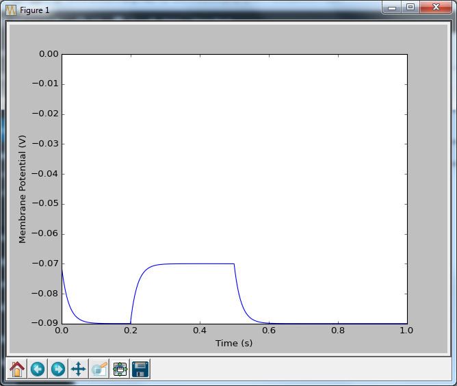Now that looks more like a neuron. A pretty dull neuron, with no action potentials, but at least we’re getting there. And how do we put in action potentials? Well we have to go and talk to two people: Hodgkin and Huxley. And we’re going to talk to them in part 2.