Recording field potentials was the first form of electrophysiology I ever did, and because of that, I tend to think that field potentials are simple. But the reality is far different. Field potentials, in my view, are harder to gain a solid understanding of than intracellular membrane potentials. So I’m going to try to take a ‘first principles’ approach to thinking about field potentials. To motivate us, I’m going to present exhibit ‘A’: The hippocampal CA1 population spike.
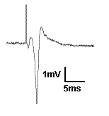
Exhibit A: A CA1 population spike. Recorded by me in 2004.
Typically, when most neuroscientists want to make an electrical model of a cell, (and prepare yourself, as there are going to be quite a few of those) they do something like this:

Typical electrical model of the cell.
 ) that has a reversal potential (
  ) and these produce currents that charge up the membrane capacitor (
  ). We literally HAVE to make the model more complex to even generate a field potential, but before we do, we’re going to simplify matters. We know those conductances create a current, which is explained with the equation:
 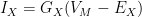 . The different currents add up linearly, giving us a total ionic current. So let’s just scrap all of these reversal potentials and conductances, and treat them as a current source. (Personally, I think this is a better way to get an intuitive understanding of membrane biophysics anyway. Membrane resistors cause people lots of confusion).
Simpler model of a cell
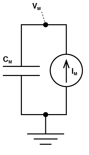
Two Compartment Model
 . The outside of each compartment is connected to ground by a resistor
  and
and  . And finally, the outside of each compartment is connected via an extracellular resistor
  .
.
Let’s imagine glutamate is released onto the dendrite, which causes AMPA channels to open. This causes an increase in 


Now that may have been a little complex. I urge you to draw the circuit yourself, and follow how the current and voltages form, however, we can make it even simpler. Let’s just explain it with words. If an EPSP forms locally, current must flow from where the membrane potential is more depolarized, to the rest of the cell, that is we get axial current. Because of the rule that the current flowing into a compartment must be equal to the current flowing out of it, when current flows into the second compartment, it must flow out of it. In a two compartment model, this means all axial current flows out into the extracellular space. Some of this current must flow back to the extracellular space where the EPSP formed initially, and some must flow to ground. The current that flowed to ground creates a positive field potential outside the second compartment. Because some of the current flowed to ground, then the current that flowed back to the extracellular space outside of where the EPSP formed is not equal to what flowed into the cell to begin with, hence some current must flow from ground to that site, to make up the difference. This creates a negative voltage, relative to ground. This concept, expanded across multiple compartments is what gives rise to “current sources” and “current sinks”, and is fully explored in “current source density experiments”. The current sink is where positive charge moves into the cell (e.g. the site of an EPSP) and a current source is where the positive charge moves out of the cell.
Below I’m simulating the field potential generated in the above two compartment model when an 5 nS EPSP impacts the dendrite. Adjust the properties of the cell to get a feel about what is happening inside and outside the cell. (Forgive the scripts slowness, each graph requires about 40,000 computations)
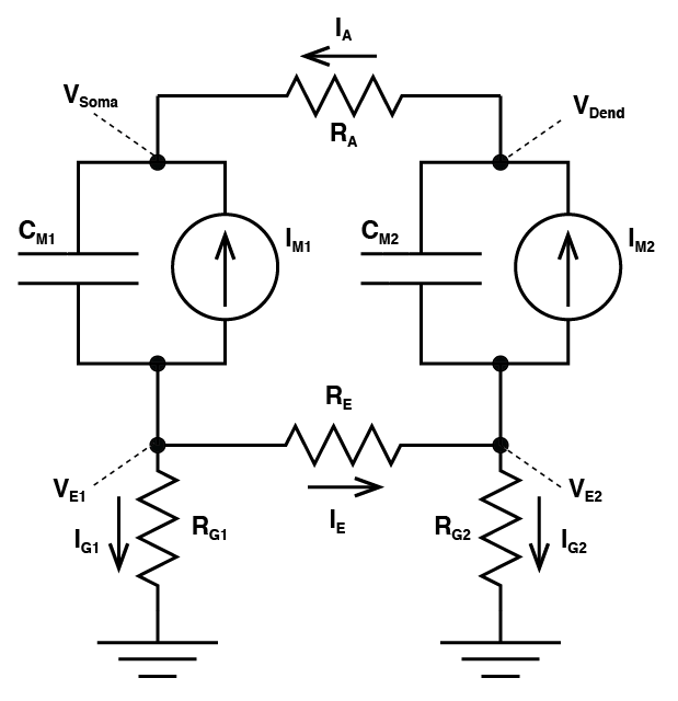
Now what you should notice is that no matter how you change the parameters of the simulation, the local field potential at the soma is equal and opposite to the field potential at the dendrite. This is a property of all two compartment simulations where the resistors to ground are equal. Exactly why that is might not be immediately apparent, but if we do simplify the circuit, we can get a feel for why that is.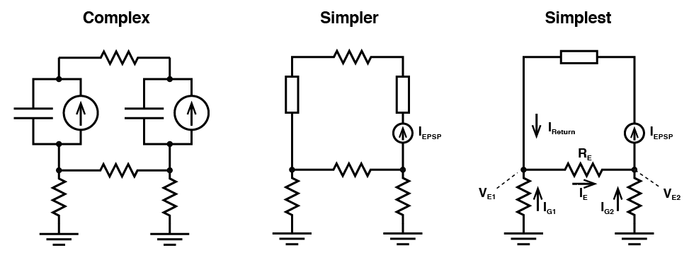 (Don’t get concerned about the direction that the arrows are pointing to show current flow. These are not meant to suggest the direction of positive charge movement. We just need to define current in some direction!)
Now we can see what is going on: Any current that flows into one compartment (


Now, this is only a two compartment model, so it will never accurately represent the complex field potentials seen in real neural tissue. But it DOES give you the fundamental insight: all current that flows into a cell must flow out of the cell at some point in space. This current then flows back to where the current moved into the cell. This extracellular current flow gives rise to the local field potential. These same ideas explain why the local field potential and EEG usually go in opposite directions and even why the signals of a multi-lead ECG look different from lead to lead.